Theory and Design

library(heteff)

Overview

heteff is built around three generalized random forest estimators:

• grf::causal_forest()
• grf::causal_survival_forest()
• grf::instrumental_forest()

The package is intentionally small. It assumes that the user has already defined an analysis table and wants a consistent way to:

1. estimate heterogeneous effects,
2. summarize the fitted forest into reusable tables,
3. expose the dominant effect modifiers through a shallow explanation tree.

The goal is not to replace grf, but to make a narrow subset of grf workflows easier to run repeatedly and easier to communicate.

Observed data and notation

For each sample $i = 1, \dots, n$, let:

• $X_i \in \mathbb{R}^p$ be a vector of baseline covariates,
• $W_i$ be treatment or exposure,
• $Y_i$ be the outcome,
• $Z_i$ be an instrument when an IV design is used.

The package works with two observed-data structures.

Observational and survival workflows

$$O_i = (Y_i, W_i, X_i)$$

The user is asserting that, conditional on $X_i$, treatment assignment is ignorable enough for a causal-forest analysis to be meaningful.

Instrumental workflow

$$O_i = (Y_i, W_i, Z_i, X_i)$$

The user is asserting that $Z_i$ is a valid instrument after conditioning on the chosen baseline covariates $X_i$.

Core estimands

Observational causal forest

The observational workflow targets the conditional average treatment effect:

$$\tau(x) = E[Y(1) - Y(0) \mid X = x].$$

This estimand asks how much expected outcome changes when treatment changes from 0 to 1, among samples with baseline profile $X = x$.

In practice, grf::causal_forest() uses orthogonalization and forest-based adaptive neighborhood weighting to estimate $\tau(x)$ without forcing the user to specify one global parametric interaction model.

Survival causal forest

For right-censored outcomes, heteff uses grf::causal_survival_forest(). At a user-specified horizon $h$, the estimand is one of:

$$\tau_{\text{RMST}}(x; h) = E[\min(T(1), h) - \min(T(0), h) \mid X = x]$$

or

$$\tau_{S}(x; h) = P(T(1) > h \mid X = x) - P(T(0) > h \mid X = x).$$

The first is a subgroup-specific restricted mean survival time difference up to horizon $h$. The second is a subgroup-specific survival-probability difference at the same horizon.

These are useful because they turn a time-to-event problem into an estimand that can be compared across clinically interpretable subgroups.

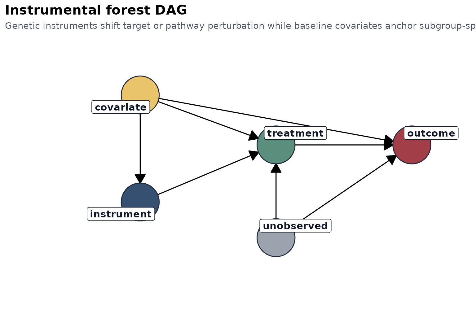
Instrumental forest

The IV workflow uses grf::instrumental_forest() and targets:

$$\tau(x) = \frac{\mathrm{Cov}(Y, Z \mid X = x)} {\mathrm{Cov}(W, Z \mid X = x)}.$$

This is the local IV effect identified by instrument-induced variation in $W$, conditional on $X = x$. When the IV assumptions hold, this quantity can be interpreted as a subgroup-specific local causal effect.

The ratio form is important:

• the numerator measures how the instrument shifts the outcome,
• the denominator measures how the instrument shifts the exposure,
• their ratio scales the reduced-form association into a local causal effect.

Design assumptions

heteff does not prove design validity. It assumes the design has already been chosen well enough that a heterogeneous-effect analysis is sensible.

Observational assumptions

For the observational and survival workflows, the main assumptions are:

1. consistency,
2. no interference,
3. conditional exchangeability given $X$,
4. overlap or positivity.

In practical terms, this means the covariate set should be baseline-only, clinically defensible, and rich enough to capture major confounding pathways.

Instrumental assumptions

For the IV workflow, the main assumptions are:

1. relevance: $Z$ shifts $W$,
2. exclusion: $Z$ affects $Y$ only through $W$,
3. instrument independence given $X$,
4. enough overlap and effective first-stage strength.

The package cannot guarantee these assumptions, but it does report a compact check_table that includes first-stage correlation and an F-statistic as a minimal diagnostic layer.

DAGs

The package ships with two compact design DAGs.

Observational DAG

plot_observational_dag()

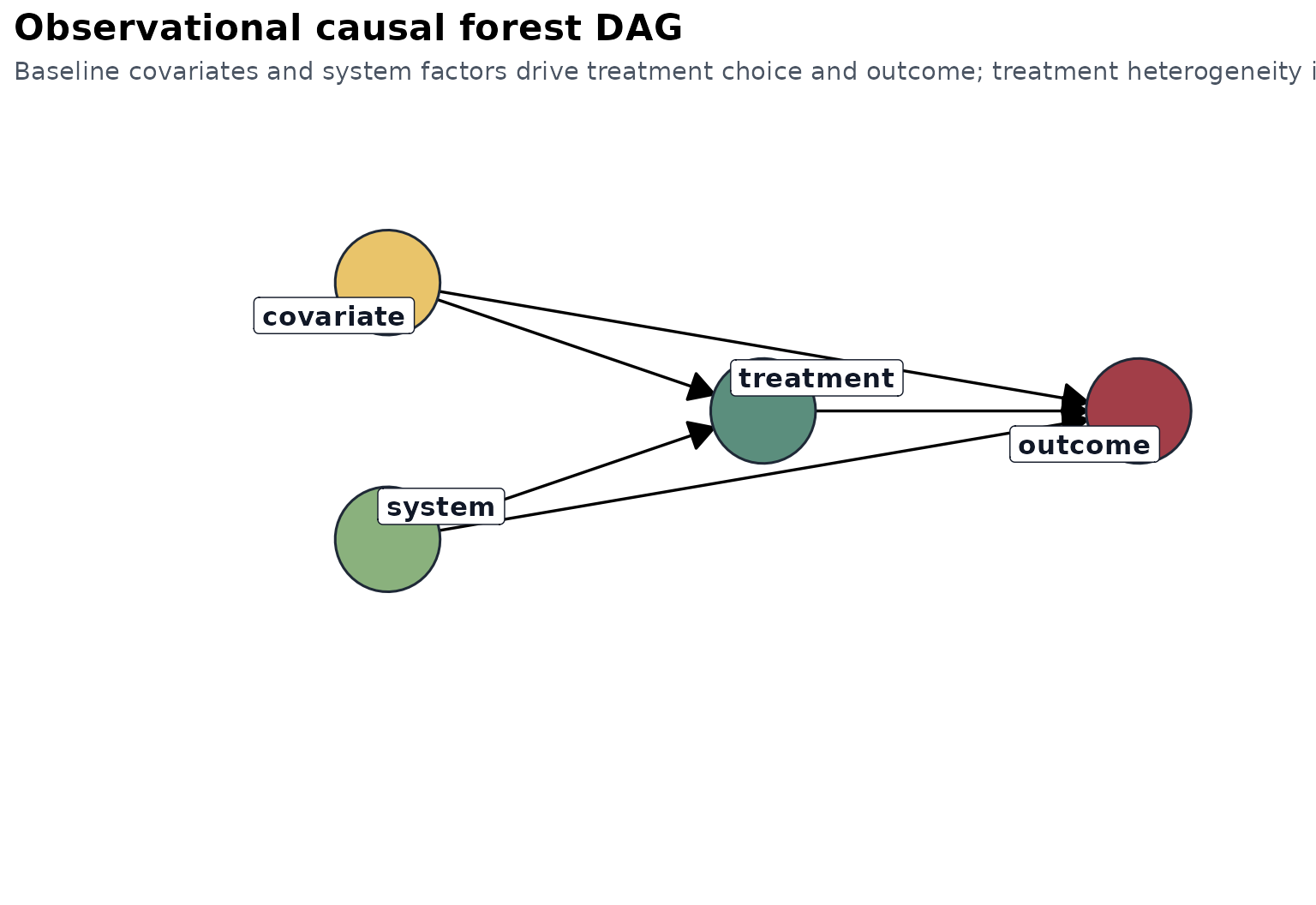
Interpretation:

• baseline covariates and system factors affect both treatment and outcome,
• the causal target is identified by adjusting for baseline $X$,
• subgroup heterogeneity is modeled as effect variation over $X$.

Instrumental DAG

plot_instrumental_dag()

Interpretation:

• unmeasured factors may jointly affect $W$ and $Y$,
• the instrument supplies exogenous variation in $W$,
• baseline covariates anchor subgroup-specific local IV effects.

What the package computes

The package-level workflow is the same across estimators.

1. Build the forest from one analysis table.
2. Predict sample-level heterogeneous effects.
3. Aggregate predicted effects into subgroup summaries.
4. Fit a shallow explanation tree to the predicted effects.
5. Rank candidates within subgroup when a candidate column is present.

This produces a shared output contract:

• effect_table
• subgroup_table
• tree_table
• ranking_table
• check_table
• estimand_table
• variable_importance

Explanation tree as a reporting layer

The explanation tree is not the forest itself. This distinction matters.

The forest is the primary estimator. It is flexible, local, and ensemble-based. The explanation tree is a secondary model fit to the predicted effects:

$$\widehat{\tau}_i = \widehat{\tau}(X_i)$$

followed by a shallow regression tree:

$$\widehat{\tau}_i \approx g(X_i).$$

This second-stage tree is used only to create readable subgroup rules. It is a communication layer, not a replacement estimand.

Why the package stays simple

The package does not attempt to expose all of grf. It stays centered on three estimators because those three correspond to three common design classes:

• treatment-effect heterogeneity in observational data,
• heterogeneous effects for right-censored survival outcomes,
• local IV heterogeneity in instrumental settings.

That constraint keeps the interface readable, the outputs stable, and the tutorials coherent.