Case Study: card.data • heteff

library(heteff)

Background

ivmodel::card.data is one of the standard teaching datasets for instrumental variables. It studies returns to schooling using college proximity as an instrument for education.

Objective

The goal is to move from a single IV estimate to a subgroup-specific local IV effect. The question becomes:

$\tau(x) = \frac{\mathrm{Cov}(Y, Z \mid X = x)} {\mathrm{Cov}(W, Z \mid X = x)},$

where $Y$ is log wage, $W$ is years of education, $Z$ is college proximity, and $X$ contains observed background variables.

Analysis setup

dat <- prepare_case_card_data()

fit <- fit_instrumental_forest(
  data = dat,
  outcome = "outcome",
  treatment = "treatment",
  instrument = "instrument",
  covariates = setdiff(names(dat), c("sample_id", "outcome", "treatment", "instrument")),
  sample_id = "sample_id",
  seed = 123,
  num_trees = 400,
  tree_minbucket = 160
)
#> Warning in get_scores.instrumental_forest(forest, subset = subset,
#> debiasing.weights = debiasing.weights, : The instrument appears to be weak,
#> with some compliance scores as low as -0.359

fit$check_table
#>                 check_name        value status
#> 1                rows_used 2220.0000000   info
#> 2     rows_dropped_missing    0.0000000     ok
#> 3               outcome_sd    0.4396932     ok
#> 4             treatment_sd    2.5877066     ok
#> 5            instrument_sd    0.4631137     ok
#> 6 cor_treatment_instrument    0.1258198     ok
#> 7            first_stage_f   35.6771160     ok
fit$subgroup_table
#>   subgroup                                     rule   n effect_mean
#> 1       G1 exper>=5.5 & fatheduc< 8.5 & exper< 11.5 499    1.110766
#> 2       G3  exper>=5.5 & fatheduc>=8.5 & exper>=8.5 226    0.536643
#> 3       G4  exper>=5.5 & fatheduc>=8.5 & exper< 8.5 306    3.070764
#> 4       G6                  exper< 5.5 & exper>=3.5 479   -2.255946
#>     effect_low effect_high
#> 1 -0.105598562    2.327130
#> 2  0.343413025    0.729873
#> 3  0.004119645    6.137409
#> 4 -6.592747148    2.080855

Design view

plot_instrumental_dag()

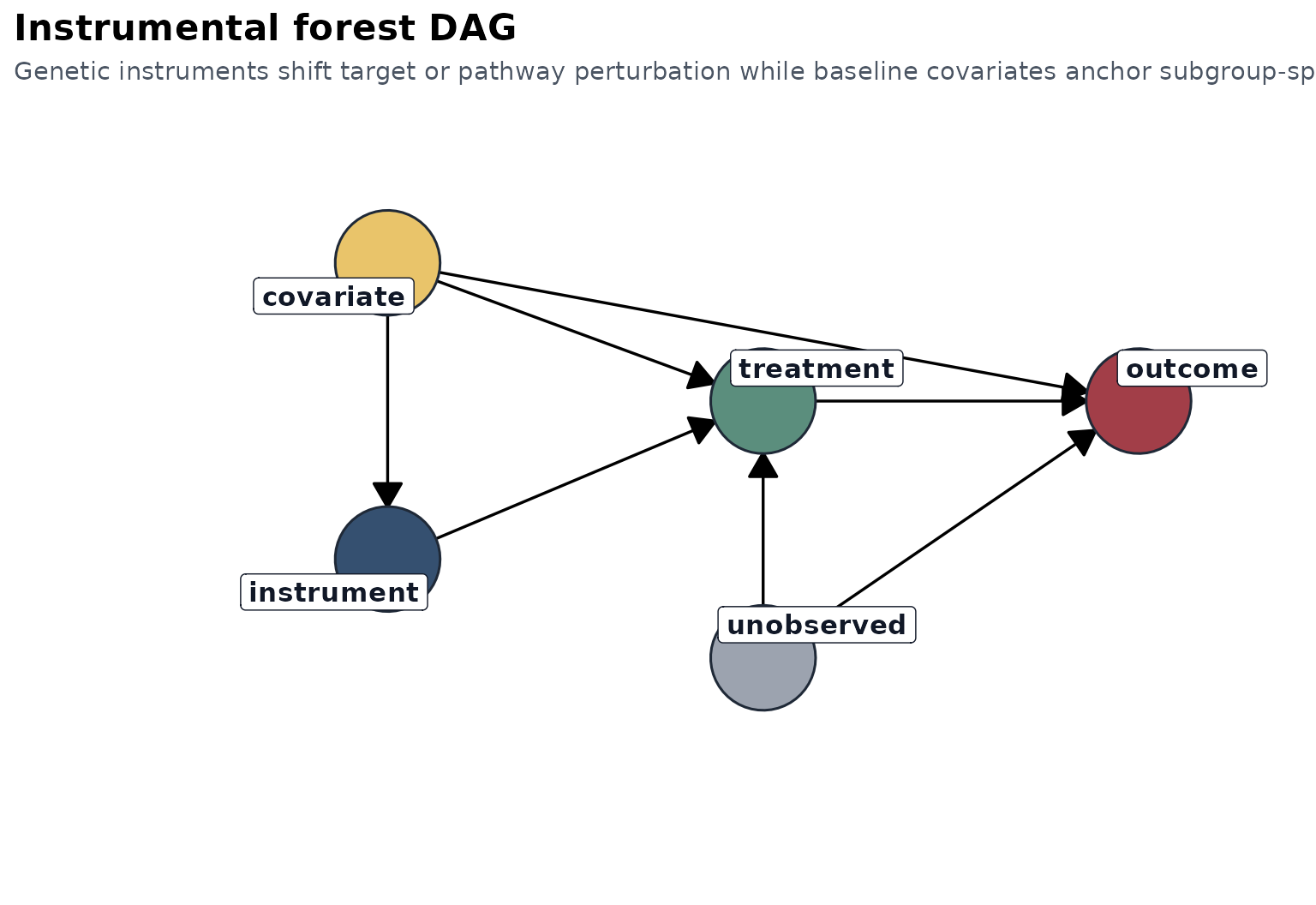
The DAG emphasizes why IV is needed: unmeasured determinants of schooling and wages can bias a naive observational effect of education.

First stage

plot_first_stage(fit)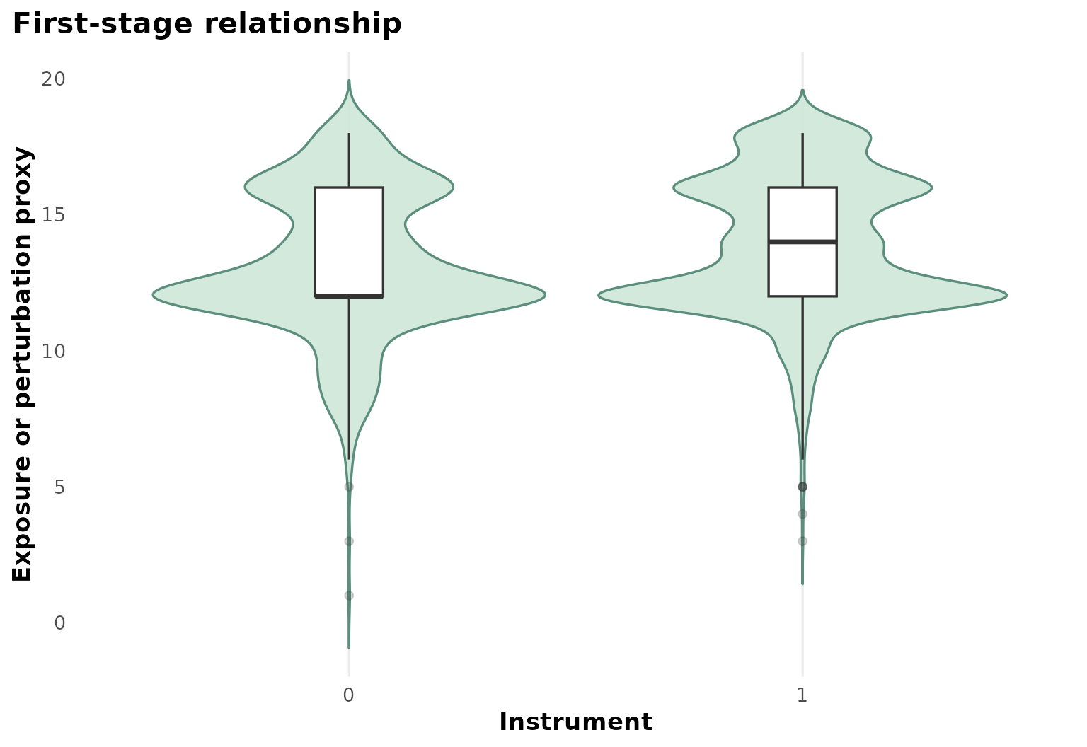

The first-stage figure shows whether the instrument visibly shifts education. This is not a full relevance analysis, but it is a useful visual complement to the first-stage F-statistic in check_table.

Reduced form

plot_reduced_form(fit)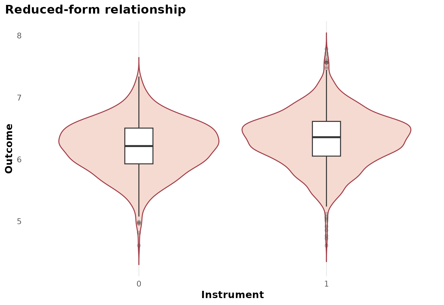

The reduced-form plot shows whether the instrument is also associated with the outcome. Together, the first-stage and reduced-form views help interpret the ratio estimand used by the instrumental forest.

Heterogeneous effect summary

plot_subgroup_effects(fit)

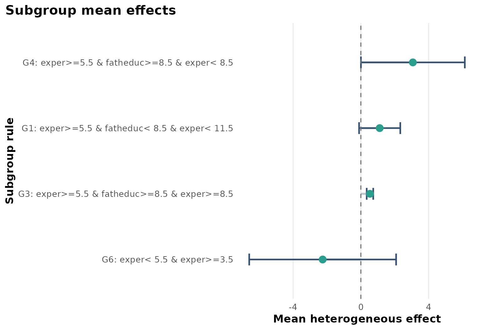
The subgroup plot shows that the local IV effect is not estimated as constant. In this example, parental education and labor-market experience help organize the heterogeneity.

Explanation tree

plot_effect_tree(fit)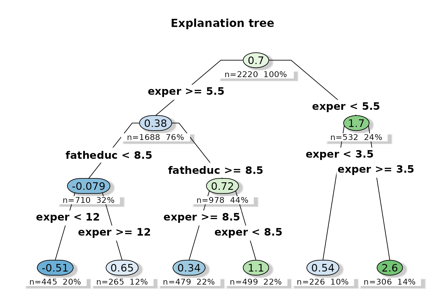

The explanation tree provides a readable summary of where the forest places its largest local-effect differences.

Variable importance

plot_variable_importance(fit)

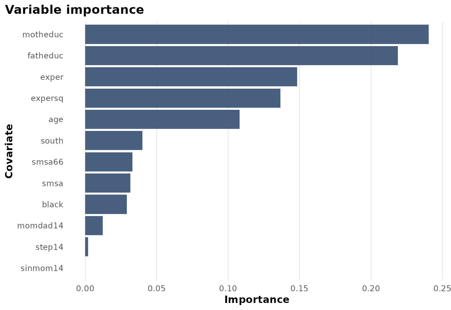
The top variables line up with an interpretable story: background advantage and experience shape where education returns appear most differentiated.

Interpretation

This case study is useful because it turns a standard IV tutorial into a heterogeneity tutorial:

the first stage is visible,
the reduced form is visible,
subgroup differences can be summarized rather than left as one global IV coefficient.

Limitations

The package still reports weak-IV warnings for some leaves in this dataset. That means subgroup interpretation should be cautious. The local IV forest is most informative as a structured exploration of heterogeneous compliance-driven effects, not as automatic evidence that every leaf is equally well identified.