Case Study: SchoolingReturns • heteff

library(heteff)

Background

ivreg::SchoolingReturns is another returns-to-schooling dataset with college proximity instruments and a richer collection of baseline socioeconomic covariates than the simpler Card example.

Objective

The purpose of this tutorial is to show the same IV workflow on a higher dimensional baseline space. The estimand is the subgroup-specific local IV effect of education on log wages.

Analysis setup

dat <- prepare_case_schooling_returns()

fit <- fit_instrumental_forest(
  data = dat,
  outcome = "outcome",
  treatment = "treatment",
  instrument = "instrument",
  covariates = setdiff(names(dat), c("sample_id", "outcome", "treatment", "instrument")),
  sample_id = "sample_id",
  seed = 123,
  num_trees = 400,
  tree_minbucket = 80
)
#> Warning in get_scores.instrumental_forest(forest, subset = subset,
#> debiasing.weights = debiasing.weights, : The instrument appears to be weak,
#> with some compliance scores as low as -0.1058

fit$check_table
#>                 check_name        value status
#> 1                rows_used 2.033000e+03   info
#> 2     rows_dropped_missing 0.000000e+00     ok
#> 3               outcome_sd 4.177972e-01     ok
#> 4             treatment_sd 2.275749e+00     ok
#> 5            instrument_sd 4.551006e-01     ok
#> 6 cor_treatment_instrument 9.353879e-02     ok
#> 7            first_stage_f 1.792710e+01     ok
fit$subgroup_table
#>   subgroup                                                 rule   n effect_mean
#> 1       G1         south66< 0.5 & meducation>=10.12 & kww< 30.5 121  -0.3156606
#> 2       G3 south66< 0.5 & meducation< 10.12 & education66>=10.5 174   0.2716612
#>   effect_low effect_high
#> 1 -3.1901339    2.558813
#> 2  0.1961033    0.347219

Design view

plot_instrumental_dag()

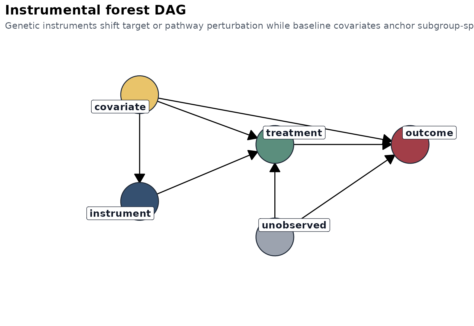
The DAG is the same IV logic as in the Card example, but the baseline covariates now allow a more detailed heterogeneity decomposition.

First stage

plot_first_stage(fit)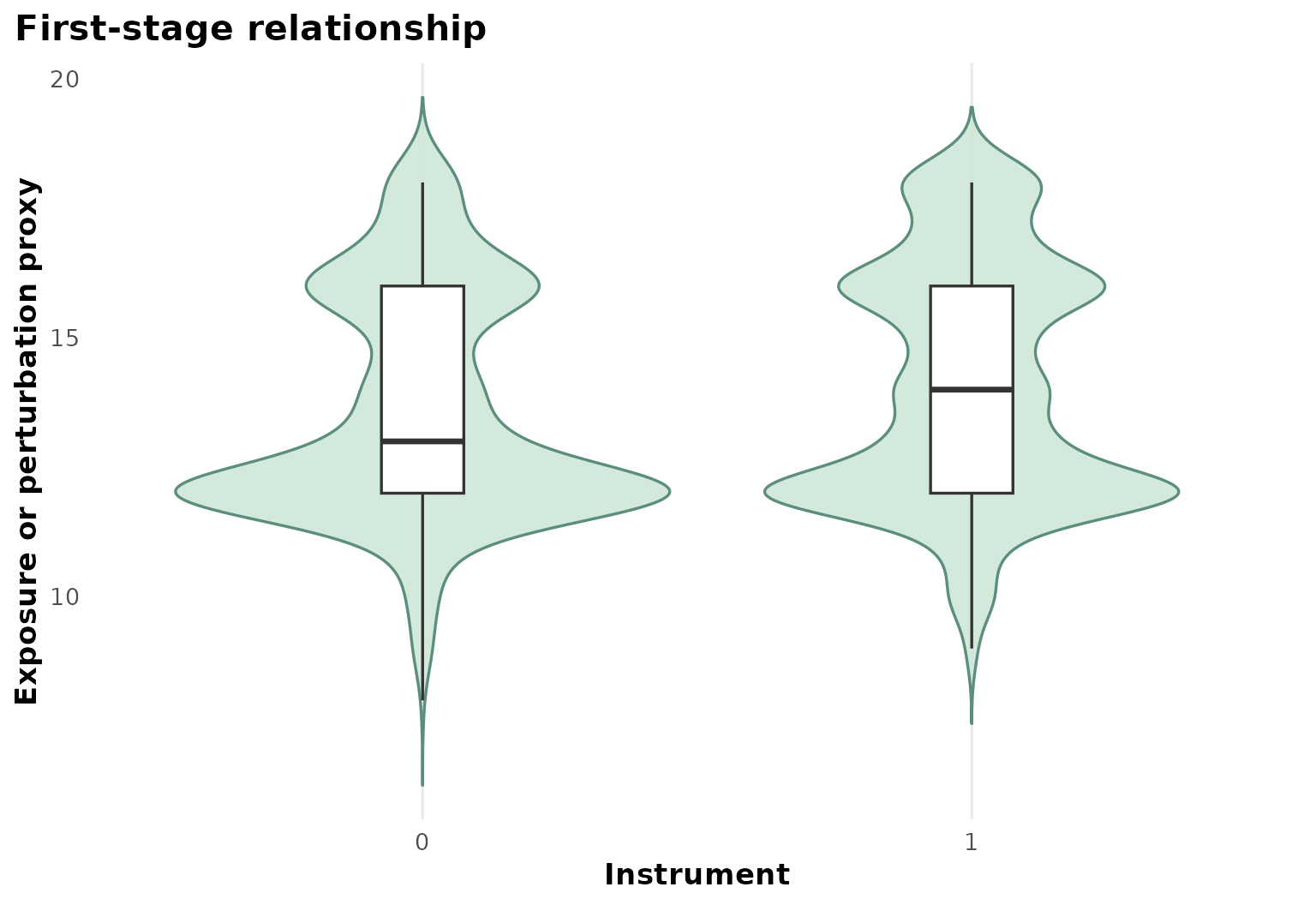

The first-stage panel shows the instrument-exposure link at the analysis-table level.

Reduced form

plot_reduced_form(fit)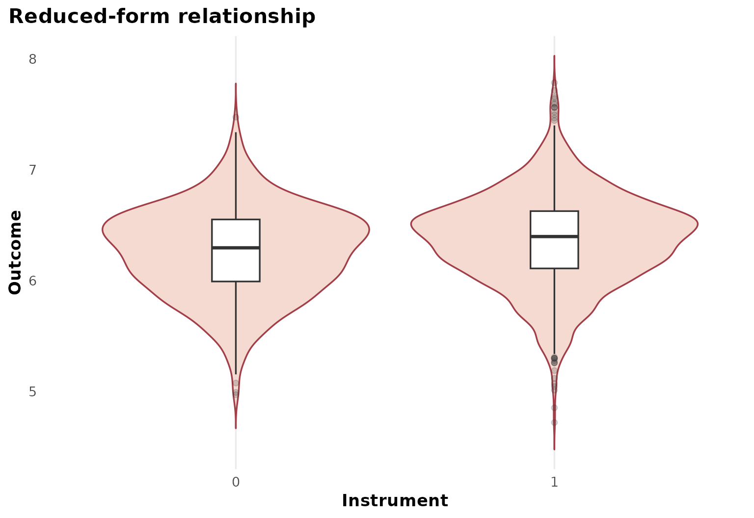

The reduced-form panel complements the first stage by showing the instrument-outcome relationship.

Heterogeneous effect summary

plot_subgroup_effects(fit)

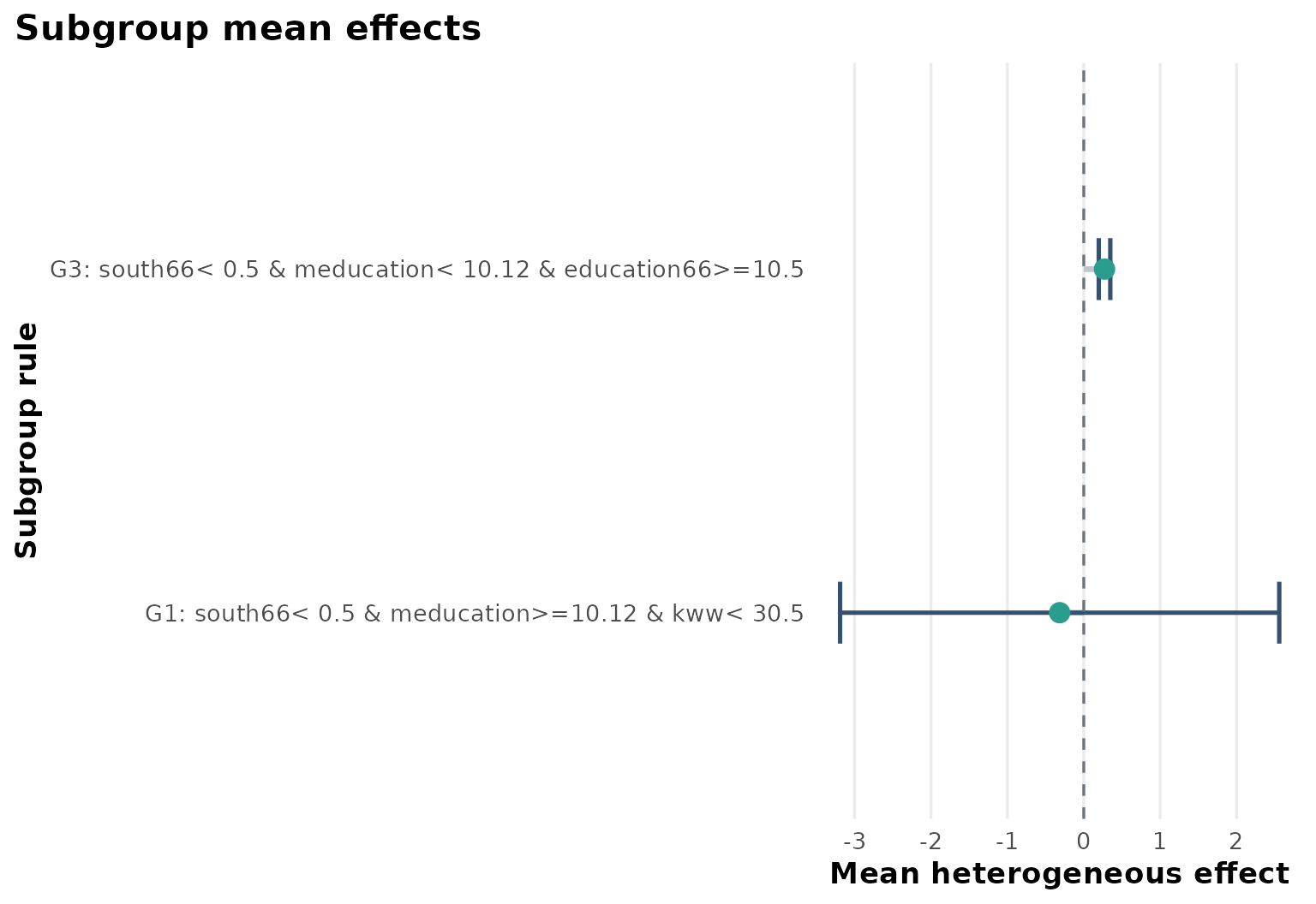
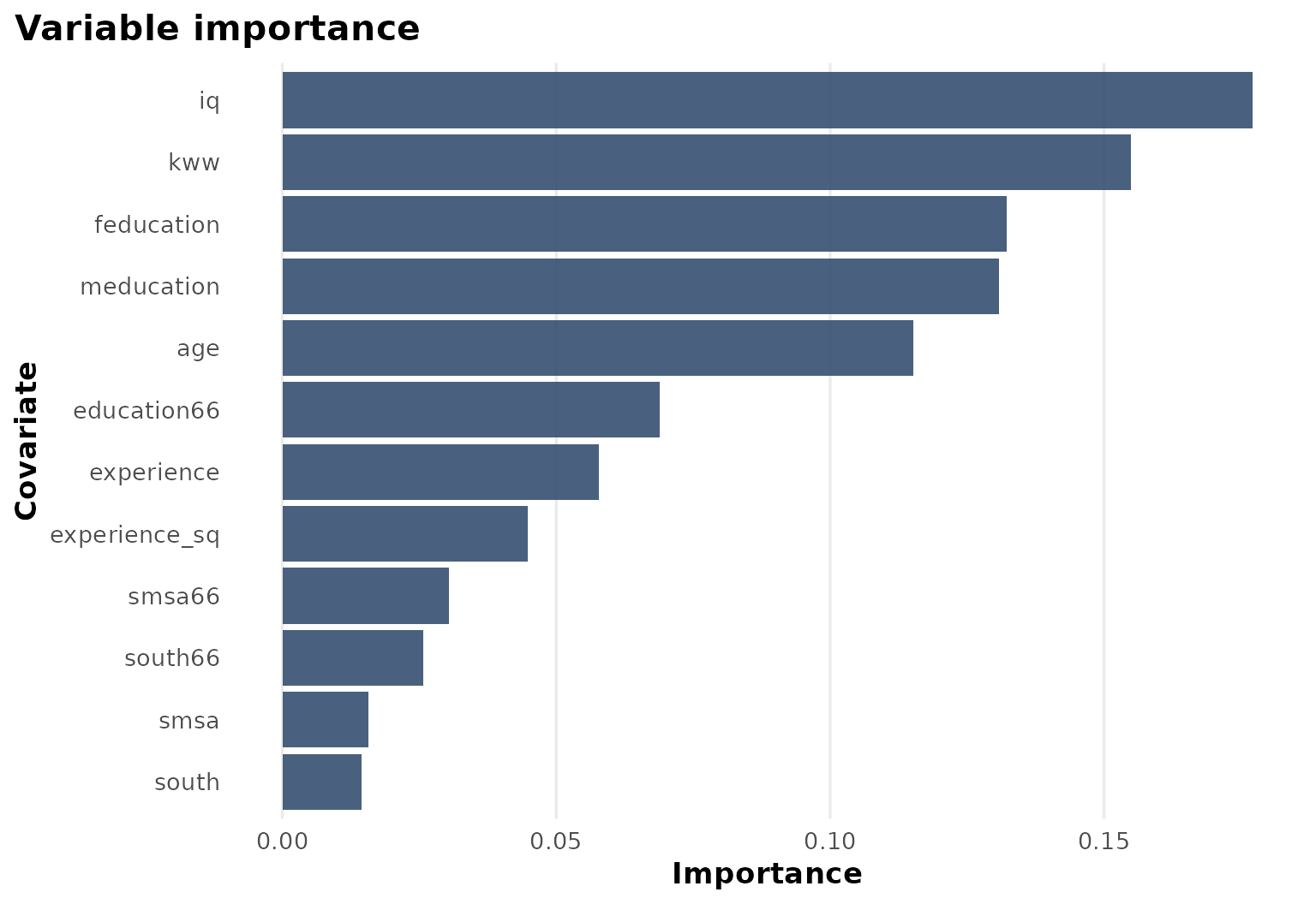
The subgroup plot suggests that local IV effects differ across baseline family education and cognitive-score profiles.

Explanation tree

plot_effect_tree(fit)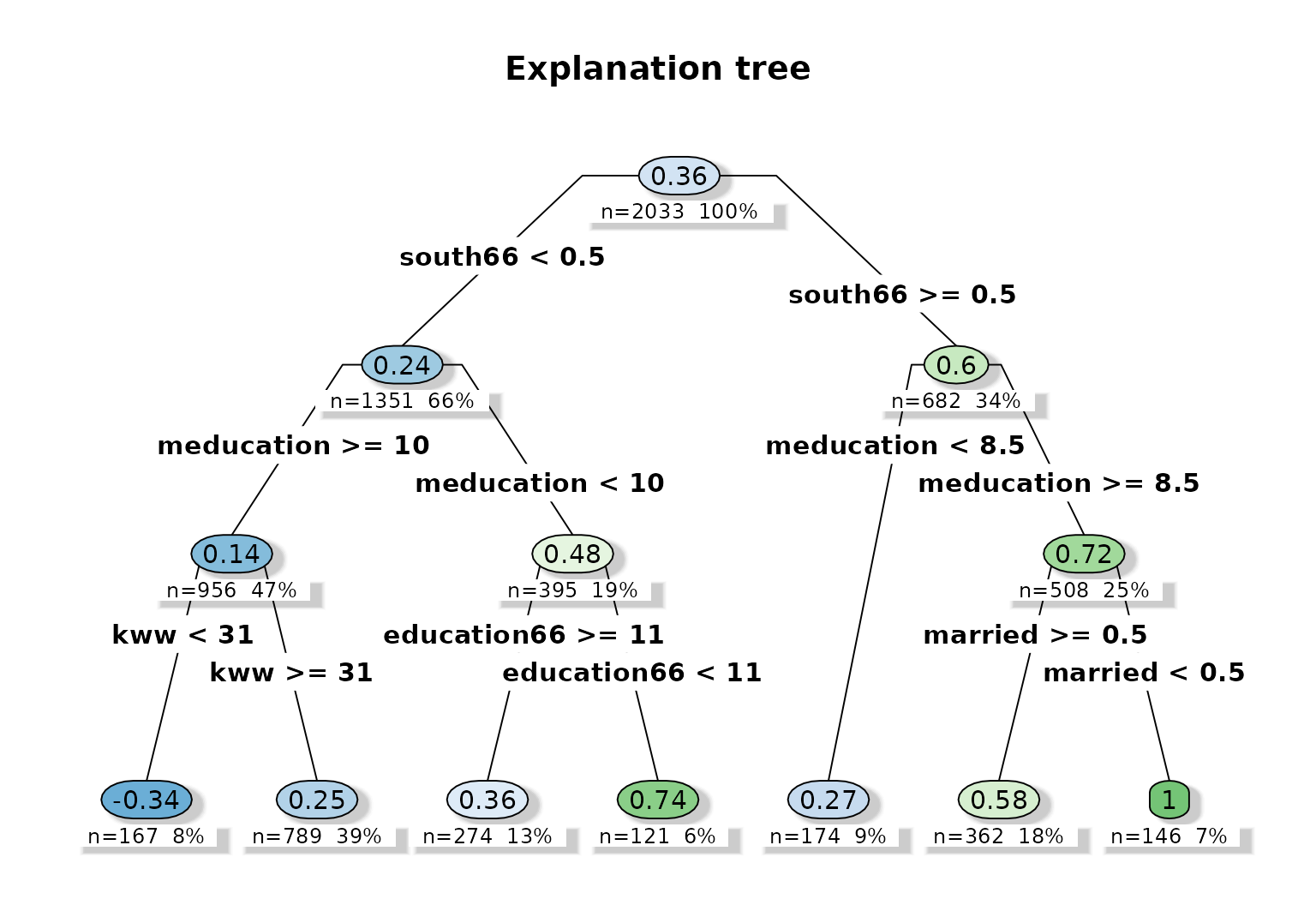

The explanation tree turns the forest predictions into readable rules. In this example, parental education, baseline schooling, and measured skill variables all contribute.

Variable importance

plot_variable_importance(fit)

The importance ranking helps connect the tree back to the full forest fit.

Interpretation

This tutorial is valuable because it shows that the instrumental workflow is not limited to one famous teaching dataset. The same logic transfers to a larger baseline space, while keeping a consistent set of outputs.

Limitations

As with any local IV analysis, interpretation depends on instrument validity and local compliance. The subgroup rules should therefore be read as summaries of where the local IV effect appears to vary, not as universal returns to schooling estimates for all populations.