Overview
This article uses the public survival::veteran dataset
as a compact real-data example. It is not a production oncology
registry, but it provides a real patient-level time-to-event dataset
with treatment assignment and baseline covariates.
Prepare the public dataset
library(survival)

data(veteran, package = "survival")
#> Warning in data(veteran, package = "survival"): data set 'veteran' not found

veteran2 <- veteran
veteran2$arm <- ifelse(veteran2$trt == 1, "SOC", "A")
veteran2$event <- veteran2$status
veteran2$subgroup <- as.character(veteran2$celltype)
veteran2$prior <- factor(veteran2$prior)

head(veteran2)
#>   trt celltype time status karno diagtime age prior arm event subgroup
#> 1   1 squamous   72      1    60        7  69     0 SOC     1 squamous
#> 2   1 squamous  411      1    70        5  64    10 SOC     1 squamous
#> 3   1 squamous  228      1    60        3  38     0 SOC     1 squamous
#> 4   1 squamous  126      1    60        9  63    10 SOC     1 squamous
#> 5   1 squamous  118      1    70       11  65    10 SOC     1 squamous
#> 6   1 squamous   10      1    20        5  49     0 SOC     1 squamous
profile_cce_dataset(
  data = veteran2,
  arm = "arm",
  time = "time",
  event = "event",
  subgroup = "subgroup"
)
#> CCE dataset profile
#>     n events event_rate median_follow_up max_follow_up
#> 1 137    128  0.9343066               80           999
Fit a VS comparison
vs_fit <- fit_cce_vs(
  data = veteran2,
  arm = "arm",
  time = "time",
  event = "event",
  covariates = c("karno", "diagtime", "age", "prior", "subgroup"),
  subgroup = "subgroup",
  tau = 180,
  landmark_times = c(90, 180),
  bootstrap = 10,
  seed = 300
)

summary(vs_fit)
#> CCE VS result
#> Label: ok
#> Warnings: Residual covariate imbalance detected.
#>   mode   method subgroup tau rmst_arm0 rmst_arm1    delta_rmst landmark_time
#> 1   vs gformula      All 180  17.42348  13.70885  -3.714629360            90
#> 2   vs gformula      All 180  17.42348  13.70885  -3.714629360           180
#> 3   vs  iptw_km      All 180  94.46028  81.83579 -12.624490041            90
#> 4   vs  iptw_km      All 180  94.46028  81.83579 -12.624490041           180
#> 5   vs iptw_cox      All 180  88.51387  88.51779   0.003925953            90
#> 6   vs iptw_cox      All 180  88.51387  88.51779   0.003925953           180
#>   survival_arm0 survival_arm1 delta_survival delta_rmst_lower_ci
#> 1   0.022844751  0.0106242942  -1.222046e-02           -9.131745
#> 2   0.001166565  0.0002869724  -8.795925e-04           -9.131745
#> 3   0.544475074  0.4012334748  -1.432416e-01          -30.010487
#> 4   0.191913854  0.2287792627   3.686541e-02          -30.010487
#> 5   0.475309651  0.4753349641   2.531322e-05          -11.082825
#> 6   0.212142801  0.2121663536   2.355226e-05          -11.082825
#>   delta_rmst_upper_ci delta_survival_lower_ci delta_survival_upper_ci
#> 1          -0.9845419            -0.039905898           -1.360854e-04
#> 2          -0.9845419            -0.024627849           -1.241037e-09
#> 3          -4.4122734            -0.272187557           -7.639318e-02
#> 4          -4.4122734            -0.006723102            9.796009e-02
#> 5           7.6966722            -0.072056221            4.926232e-02
#> 6           7.6966722            -0.062511997            4.403169e-02
plot(vs_fit, method = "iptw_km", subgroup = "All")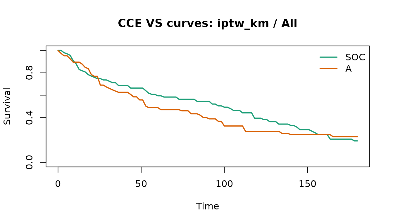
head(as_effects_df(vs_fit))
#>   mode   method subgroup tau rmst_arm0 rmst_arm1    delta_rmst landmark_time
#> 1   vs gformula      All 180  17.42348  13.70885  -3.714629360            90
#> 2   vs gformula      All 180  17.42348  13.70885  -3.714629360           180
#> 3   vs  iptw_km      All 180  94.46028  81.83579 -12.624490041            90
#> 4   vs  iptw_km      All 180  94.46028  81.83579 -12.624490041           180
#> 5   vs iptw_cox      All 180  88.51387  88.51779   0.003925953            90
#> 6   vs iptw_cox      All 180  88.51387  88.51779   0.003925953           180
#>   survival_arm0 survival_arm1 delta_survival delta_rmst_lower_ci
#> 1   0.022844751  0.0106242942  -1.222046e-02           -9.131745
#> 2   0.001166565  0.0002869724  -8.795925e-04           -9.131745
#> 3   0.544475074  0.4012334748  -1.432416e-01          -30.010487
#> 4   0.191913854  0.2287792627   3.686541e-02          -30.010487
#> 5   0.475309651  0.4753349641   2.531322e-05          -11.082825
#> 6   0.212142801  0.2121663536   2.355226e-05          -11.082825
#>   delta_rmst_upper_ci delta_survival_lower_ci delta_survival_upper_ci
#> 1          -0.9845419            -0.039905898           -1.360854e-04
#> 2          -0.9845419            -0.024627849           -1.241037e-09
#> 3          -4.4122734            -0.272187557           -7.639318e-02
#> 4          -4.4122734            -0.006723102            9.796009e-02
#> 5           7.6966722            -0.072056221            4.926232e-02
#> 6           7.6966722            -0.062511997            4.403169e-02
Create an SOC-only projection
For scenario planning, we can keep only the SOC rows and overlay assumption-based proportional-hazards projections.
soc_fit <- project_soc_only(
  data = veteran2,
  arm = "arm",
  soc_level = "SOC",
  time = "time",
  event = "event",
  subgroup = "subgroup",
  tau = 180,
  hr_scenarios = c(0.75, 0.90, 1.00),
  target_delta_rmst = 15,
  prior_mean_log_hr = log(0.85),
  prior_sd_log_hr = 0.20,
  bootstrap = 10,
  seed = 400
)

summary(soc_fit)
#> CCE SOC-only projection
#> Label: Projection (assumption-based)
#>       mode        method subgroup scenario_hr tau rmst_arm0 rmst_arm1
#> 1 soc_only projection_ph      All        0.75 180  96.12878 110.83745
#> 2 soc_only projection_ph      All        0.75 180  96.12878 110.83745
#> 3 soc_only projection_ph      All        0.90 180  96.12878 101.65283
#> 4 soc_only projection_ph      All        0.90 180  96.12878 101.65283
#> 5 soc_only projection_ph      All        1.00 180  96.12878  96.12878
#> 6 soc_only projection_ph      All        1.00 180  96.12878  96.12878
#>   delta_rmst landmark_time survival_arm0 survival_arm1 delta_survival
#> 1  14.708678            90     0.5467462     0.6358276     0.08908133
#> 2  14.708678           180     0.2124268     0.3129010     0.10047422
#> 3   5.524058            90     0.5467462     0.5807741     0.03402784
#> 4   5.524058           180     0.2124268     0.2480209     0.03559415
#> 5   0.000000            90     0.5467462     0.5467462     0.00000000
#> 6   0.000000           180     0.2124268     0.2124268     0.00000000
#>   required_hr pos_proxy delta_rmst_lower_ci delta_rmst_upper_ci
#> 1   0.7455392     0.258           13.485943           15.473156
#> 2   0.7455392     0.258           13.485943           15.473156
#> 3   0.7455392     0.258            5.116966            5.797128
#> 4   0.7455392     0.258            5.116966            5.797128
#> 5   0.7455392     0.258            0.000000            0.000000
#> 6   0.7455392     0.258            0.000000            0.000000
#>   delta_survival_lower_ci delta_survival_upper_ci
#> 1              0.07880162              0.09380862
#> 2              0.08812526              0.10462482
#> 3              0.03039300              0.03562514
#> 4              0.03010239              0.03781181
#> 5              0.00000000              0.00000000
#> 6              0.00000000              0.00000000
plot(soc_fit, subgroup = "All")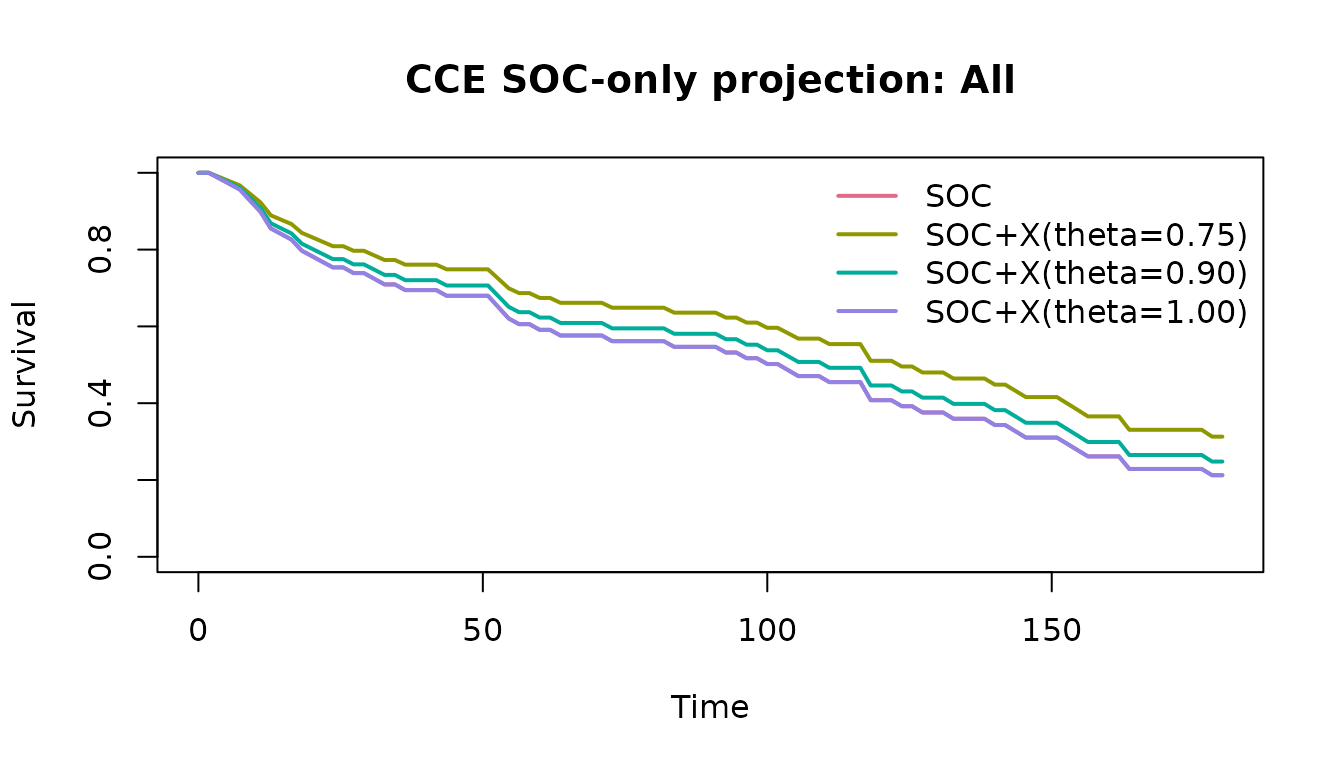
Interpretation notes
- VS-mode results include
gformula,iptw_km, andiptw_cox, so the method label should be interpreted explicitly. - SOC-only outputs are projections, not causal estimates.
- In real programs, diagnostics should be interpreted together with data provenance, treatment policy definitions, and endpoint adjudication rules.