Overview
This article shows the full CCE workflow on bundled synthetic data:
- create normalized source tables
- validate the source tables before assembly
- build an analysis-ready cohort
- estimate a VS-mode comparison
- run SOC-only projection scenarios
- export results for reporting
Generate the example data
demo <- cce_demo_data(n = 240, seed = 42)
names(demo)
#> [1] "patient_baseline"   "treatment_episodes" "outcomes"
#> [4] "biomarkers"         "spec"               "analysis_data"
The demo generator returns the four normalized tables plus a ready-made analysis dataset.
str(demo$analysis_data)
#> Classes 'cce_dataset' and 'data.frame':  240 obs. of  13 variables:
#>  $ patient_id         : chr  "P0001" "P0002" "P0003" "P0004" ...
#>  $ index_date         : Date, format: "2022-02-18" "2022-03-06" ...
#>  $ age                : num  68 65 72 62 72 48 79 72 63 51 ...
#>  $ sex                : chr  "F" "F" "F" "M" ...
#>  $ histology          : chr  "Adenocarcinoma" "Squamous" "Adenocarcinoma" "Adenocarcinoma" ...
#>  $ stage_or_risk      : chr  "III" "IV" "IV" "IV" ...
#>  $ ps                 : int  0 2 0 0 1 1 2 1 0 0 ...
#>  $ arm                : Factor w/ 2 levels "SOC","A": 2 1 2 1 1 1 2 1 1 2 ...
#>  $ start_date         : Date, format: "2022-02-18" "2022-03-06" ...
#>  $ time               : num  371 12 212 107 296 78 53 121 9 270 ...
#>  $ event              : int  1 1 0 1 1 1 1 1 1 1 ...
#>  $ last_follow_up_date: Date, format: "2023-02-24" "2022-03-18" ...
#>  $ subgroup           : chr  "High" "Low" "Low" "Low" ...
#>  - attr(*, "spec")=List of 18
#>   ..$ covariates                 : chr [1:4] "age" "sex" "stage_or_risk" "ps"
#>   ..$ subgroup_biomarker         : chr "PDL1"
#>   ..$ endpoint                   : chr "os"
#>   ..$ id_col                     : chr "patient_id"
#>   ..$ index_date_col             : chr "index_date"
#>   ..$ regimen_col                : chr "regimen_name"
#>   ..$ treatment_start_col        : chr "start_date"
#>   ..$ index_flag_col             : chr "is_index_treatment"
#>   ..$ endpoint_col               : chr "endpoint"
#>   ..$ time_col                   : chr "time"
#>   ..$ event_col                  : chr "event"
#>   ..$ follow_up_col              : chr "last_follow_up_date"
#>   ..$ biomarker_name_col         : chr "biomarker_name"
#>   ..$ biomarker_value_col        : chr "biomarker_value"
#>   ..$ biomarker_baseline_flag_col: chr "is_baseline"
#>   ..$ arm_map                    : Named chr [1:2] "SOC" "A"
#>   .. ..- attr(*, "names")= chr [1:2] "SOC" "A"
#>   ..$ missing_strategy           : chr "complete_case"
#>   ..$ time_zero_tolerance_days   : int 0
#>   ..- attr(*, "class")= chr "cce_spec"
#>  - attr(*, "exclusions")='data.frame':   1 obs. of  2 variables:
#>   ..$ reason: chr "missing_required_fields"
#>   ..$ n     : int 0
#>  - attr(*, "validation_report")='data.frame':    0 obs. of  4 variables:
#>   ..$ component: chr(0)
#>   ..$ severity : chr(0)
#>   ..$ issue    : chr(0)
#>   ..$ n        : num(0)
#>  - attr(*, "profile")=List of 5
#>   ..$ overall        :'data.frame':  1 obs. of  5 variables:
#>   .. ..$ n               : int 240
#>   .. ..$ events          : int 157
#>   .. ..$ event_rate      : num 0.654
#>   .. ..$ median_follow_up: num 218
#>   .. ..$ max_follow_up   : num 705
#>   ..$ by_arm         :'data.frame':  2 obs. of  4 variables:
#>   .. ..$ arm       : chr [1:2] "A" "SOC"
#>   .. ..$ n         : int [1:2] 110 130
#>   .. ..$ events    : int [1:2] 65 92
#>   .. ..$ event_rate: num [1:2] 0.591 0.708
#>   ..$ by_subgroup    :'data.frame':  2 obs. of  4 variables:
#>   .. ..$ subgroup  : chr [1:2] "High" "Low"
#>   .. ..$ n         : int [1:2] 129 111
#>   .. ..$ events    : int [1:2] 78 79
#>   .. ..$ event_rate: num [1:2] 0.605 0.712
#>   ..$ by_arm_subgroup:'data.frame':  4 obs. of  5 variables:
#>   .. ..$ arm       : chr [1:4] "A" "A" "SOC" "SOC"
#>   .. ..$ subgroup  : chr [1:4] "High" "Low" "High" "Low"
#>   .. ..$ n         : int [1:4] 53 57 76 54
#>   .. ..$ events    : int [1:4] 26 39 52 40
#>   .. ..$ event_rate: num [1:4] 0.491 0.684 0.684 0.741
#>   ..$ missingness    :'data.frame':  13 obs. of  3 variables:
#>   .. ..$ column      : chr [1:13] "patient_id" "index_date" "age" "sex" ...
#>   .. ..$ missing_n   : num [1:13] 0 0 0 0 0 0 0 0 0 0 ...
#>   .. ..$ missing_rate: num [1:13] 0 0 0 0 0 0 0 0 0 0 ...
#>   ..- attr(*, "class")= chr "cce_profile"
Round-trip the analysis specification
spec_path <- tempfile(fileext = ".yml")
write_cce_spec(demo$spec, spec_path)
roundtrip_spec <- read_cce_spec(spec_path)
roundtrip_spec$covariates
#> [1] "age"           "sex"           "stage_or_risk" "ps"
Rebuild the analysis dataset from normalized tables
validate_cce_tables(
  patient_baseline = demo$patient_baseline,
  treatment_episodes = demo$treatment_episodes,
  outcomes = demo$outcomes,
  biomarkers = demo$biomarkers,
  spec = roundtrip_spec
)
#> [1] component severity  issue     n
#> <0 rows> (or 0-length row.names)
analysis <- build_analysis_dataset(
  patient_baseline = demo$patient_baseline,
  treatment_episodes = demo$treatment_episodes,
  outcomes = demo$outcomes,
  biomarkers = demo$biomarkers,
  spec = roundtrip_spec
)

head(analysis)
#>   patient_id index_date age sex      histology stage_or_risk ps arm start_date
#> 1      P0001 2022-02-18  68   F Adenocarcinoma           III  0   A 2022-02-18
#> 2      P0002 2022-03-06  65   F       Squamous            IV  2 SOC 2022-03-06
#> 3      P0003 2022-06-02  72   F Adenocarcinoma            IV  0   A 2022-06-02
#> 4      P0004 2022-03-15  62   M Adenocarcinoma            IV  0 SOC 2022-03-15
#> 5      P0005 2022-05-26  72   M Adenocarcinoma            IV  1 SOC 2022-05-26
#> 6      P0006 2022-05-02  48   M Adenocarcinoma            IV  1 SOC 2022-05-02
#>   time event last_follow_up_date subgroup
#> 1  371     1          2023-02-24     High
#> 2   12     1          2022-03-18      Low
#> 3  212     0          2022-12-31      Low
#> 4  107     1          2022-06-30      Low
#> 5  296     1          2023-03-18     High
#> 6   78     1          2022-07-19      Low
profile_cce_dataset(
  data = analysis,
  arm = "arm",
  time = "time",
  event = "event",
  subgroup = "subgroup"
)
#> CCE dataset profile
#>     n events event_rate median_follow_up max_follow_up
#> 1 240    157  0.6541667              218           705
VS-mode estimation
vs_fit <- fit_cce_vs(
  data = analysis,
  arm = "arm",
  time = "time",
  event = "event",
  covariates = c("age", "sex", "stage_or_risk", "ps"),
  subgroup = "subgroup",
  tau = 365,
  landmark_times = c(180, 365),
  bootstrap = 20,
  seed = 100
)

summary(vs_fit)
#> CCE VS result
#> Label: ok
#> Warnings: none
#>   mode   method subgroup tau rmst_arm0 rmst_arm1 delta_rmst landmark_time
#> 1   vs gformula      All 365  188.1689  229.3371   41.16822           180
#> 2   vs gformula      All 365  188.1689  229.3371   41.16822           365
#> 3   vs  iptw_km      All 365  205.7951  259.6433   53.84820           180
#> 4   vs  iptw_km      All 365  205.7951  259.6433   53.84820           365
#> 5   vs iptw_cox      All 365  212.9197  250.6222   37.70248           180
#> 6   vs iptw_cox      All 365  212.9197  250.6222   37.70248           365
#>   survival_arm0 survival_arm1 delta_survival delta_rmst_lower_ci
#> 1     0.4739779     0.6057646      0.1317867           10.780157
#> 2     0.2492317     0.3914337      0.1422019           10.780157
#> 3     0.5143146     0.7197778      0.2054632           -6.929098
#> 4     0.3307018     0.4798347      0.1491330           -6.929098
#> 5     0.5536321     0.6708851      0.1172530            9.650522
#> 6     0.3328632     0.4758616      0.1429984            9.650522
#>   delta_rmst_upper_ci delta_survival_lower_ci delta_survival_upper_ci
#> 1            51.67511             0.032575899               0.1572542
#> 2            51.67511             0.012879768               0.1960966
#> 3            72.52610             0.003351216               0.2710959
#> 4            72.52610             0.031542439               0.2356857
#> 5            55.57671             0.031029790               0.1685626
#> 6            55.57671             0.034438024               0.2109653
plot(vs_fit, method = "gformula", subgroup = "All")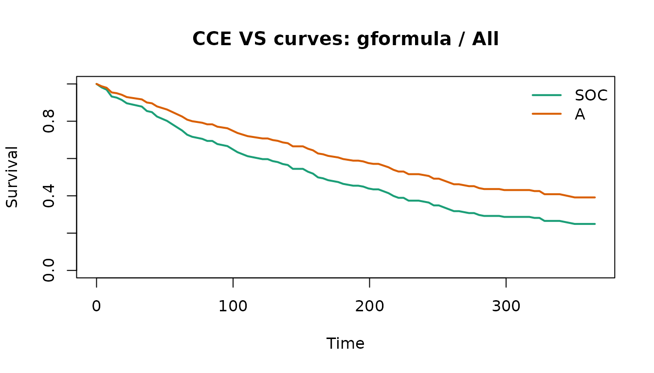
The tidy effects table is designed to feed downstream reports or dashboards.
head(as_effects_df(vs_fit))
#>   mode   method subgroup tau rmst_arm0 rmst_arm1 delta_rmst landmark_time
#> 1   vs gformula      All 365  188.1689  229.3371   41.16822           180
#> 2   vs gformula      All 365  188.1689  229.3371   41.16822           365
#> 3   vs  iptw_km      All 365  205.7951  259.6433   53.84820           180
#> 4   vs  iptw_km      All 365  205.7951  259.6433   53.84820           365
#> 5   vs iptw_cox      All 365  212.9197  250.6222   37.70248           180
#> 6   vs iptw_cox      All 365  212.9197  250.6222   37.70248           365
#>   survival_arm0 survival_arm1 delta_survival delta_rmst_lower_ci
#> 1     0.4739779     0.6057646      0.1317867           10.780157
#> 2     0.2492317     0.3914337      0.1422019           10.780157
#> 3     0.5143146     0.7197778      0.2054632           -6.929098
#> 4     0.3307018     0.4798347      0.1491330           -6.929098
#> 5     0.5536321     0.6708851      0.1172530            9.650522
#> 6     0.3328632     0.4758616      0.1429984            9.650522
#>   delta_rmst_upper_ci delta_survival_lower_ci delta_survival_upper_ci
#> 1            51.67511             0.032575899               0.1572542
#> 2            51.67511             0.012879768               0.1960966
#> 3            72.52610             0.003351216               0.2710959
#> 4            72.52610             0.031542439               0.2356857
#> 5            55.57671             0.031029790               0.1685626
#> 6            55.57671             0.034438024               0.2109653
Diagnostics are returned in a machine-readable table.
head(as_diagnostics_df(vs_fit))
#>    method subgroup             metric        value threshold  status
#> 1 iptw_km      All         max_weight   1.30235194      50.0      ok
#> 2 iptw_km      All          ess_total 238.61717626        NA    info
#> 3 iptw_km      All           ess_arm0 129.23701922        NA    info
#> 4 iptw_km      All           ess_arm1 109.38039627        NA    info
#> 5 iptw_km      All max_abs_smd_before   0.12160316       0.1 warning
#> 6 iptw_km      All  max_abs_smd_after   0.00168784       0.1      ok
SOC-only projection
soc_fit <- project_soc_only(
  data = analysis,
  arm = "arm",
  soc_level = "SOC",
  time = "time",
  event = "event",
  subgroup = "subgroup",
  tau = 365,
  hr_scenarios = c(0.65, 0.80, 1.00),
  target_delta_rmst = 30,
  prior_mean_log_hr = log(0.8),
  prior_sd_log_hr = 0.25,
  bootstrap = 20,
  seed = 200
)

summary(soc_fit)
#> CCE SOC-only projection
#> Label: Projection (assumption-based)
#>       mode        method subgroup scenario_hr tau rmst_arm0 rmst_arm1
#> 1 soc_only projection_ph      All        0.65 365  205.9825  248.3459
#> 2 soc_only projection_ph      All        0.65 365  205.9825  248.3459
#> 3 soc_only projection_ph      All        0.80 365  205.9825  228.8191
#> 4 soc_only projection_ph      All        0.80 365  205.9825  228.8191
#> 5 soc_only projection_ph      All        1.00 365  205.9825  205.9825
#> 6 soc_only projection_ph      All        1.00 365  205.9825  205.9825
#>   delta_rmst landmark_time survival_arm0 survival_arm1 delta_survival
#> 1   42.36347           182     0.5076923     0.6436361     0.13594377
#> 2   42.36347           365     0.3320886     0.4884444     0.15635574
#> 3   22.83660           182     0.5076923     0.5814073     0.07371497
#> 4   22.83660           365     0.3320886     0.4140027     0.08191410
#> 5    0.00000           182     0.5076923     0.5076923     0.00000000
#> 6    0.00000           365     0.3320886     0.3320886     0.00000000
#>   required_hr pos_proxy delta_rmst_lower_ci delta_rmst_upper_ci
#> 1   0.7429734     0.384            37.70481            45.06949
#> 2   0.7429734     0.384            37.70481            45.06949
#> 3   0.7429734     0.384            20.54640            24.13302
#> 4   0.7429734     0.384            20.54640            24.13302
#> 5   0.7429734     0.384             0.00000             0.00000
#> 6   0.7429734     0.384             0.00000             0.00000
#>   delta_survival_lower_ci delta_survival_upper_ci
#> 1              0.11746102              0.14767173
#> 2              0.15199173              0.15724805
#> 3              0.06453981              0.07902597
#> 4              0.07934582              0.08192000
#> 5              0.00000000              0.00000000
#> 6              0.00000000              0.00000000
plot(soc_fit, subgroup = "All")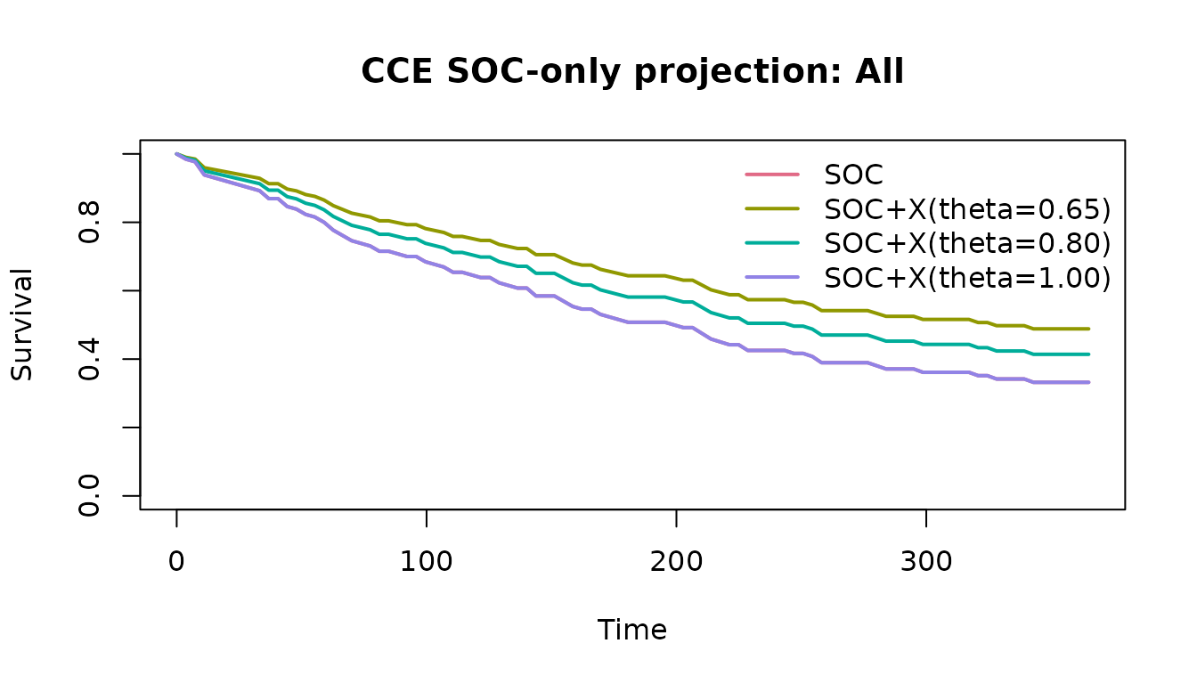
head(as_effects_df(soc_fit))
#>       mode        method subgroup scenario_hr tau rmst_arm0 rmst_arm1
#> 1 soc_only projection_ph      All        0.65 365  205.9825  248.3459
#> 2 soc_only projection_ph      All        0.65 365  205.9825  248.3459
#> 3 soc_only projection_ph      All        0.80 365  205.9825  228.8191
#> 4 soc_only projection_ph      All        0.80 365  205.9825  228.8191
#> 5 soc_only projection_ph      All        1.00 365  205.9825  205.9825
#> 6 soc_only projection_ph      All        1.00 365  205.9825  205.9825
#>   delta_rmst landmark_time survival_arm0 survival_arm1 delta_survival
#> 1   42.36347           182     0.5076923     0.6436361     0.13594377
#> 2   42.36347           365     0.3320886     0.4884444     0.15635574
#> 3   22.83660           182     0.5076923     0.5814073     0.07371497
#> 4   22.83660           365     0.3320886     0.4140027     0.08191410
#> 5    0.00000           182     0.5076923     0.5076923     0.00000000
#> 6    0.00000           365     0.3320886     0.3320886     0.00000000
#>   required_hr pos_proxy delta_rmst_lower_ci delta_rmst_upper_ci
#> 1   0.7429734     0.384            37.70481            45.06949
#> 2   0.7429734     0.384            37.70481            45.06949
#> 3   0.7429734     0.384            20.54640            24.13302
#> 4   0.7429734     0.384            20.54640            24.13302
#> 5   0.7429734     0.384             0.00000             0.00000
#> 6   0.7429734     0.384             0.00000             0.00000
#>   delta_survival_lower_ci delta_survival_upper_ci
#> 1              0.11746102              0.14767173
#> 2              0.15199173              0.15724805
#> 3              0.06453981              0.07902597
#> 4              0.07934582              0.08192000
#> 5              0.00000000              0.00000000
#> 6              0.00000000              0.00000000
Export files
out_dir <- tempfile(pattern = "cce-demo-")
write_cce_results(vs_fit, out_dir)
list.files(out_dir)
#> [1] "curves.csv"      "diagnostics.csv" "effects.csv"     "results.json"
The written directory contains:
results.jsoncurves.csveffects.csvdiagnostics.csv
results.json also stores the covariate set, threshold
settings, source spec, exclusion summary, and dataset profile for
auditability.
Notes
The bundled demo is useful for package validation and documentation.
For public patient-level data, see the companion article on
survival::veteran.