Indometh

Background

Indometh is a pharmacokinetic dataset tracking indomethacin concentration over time in several subjects. It is a compact medical-style table where assay values and subject metadata naturally mix. The repeated-measures structure makes it a useful stress test because concentration is expected to change over time, but subject-to-subject variation still matters.

Objective

The aim is to see whether uccdf can recover stable concentration-profile regimes using concentration, subject identity, and a coarse time band. The real question is whether the output looks like a meaningful stratification of the concentration curve, instead of collapsing to subject labels or to a trivial early-versus-late split.

Data preparation

ind_df <- Indometh
ind_df$sample_id <- sprintf("IN%03d", seq_len(nrow(ind_df)))
ind_df$Subject <- factor(ind_df$Subject)
ind_df$time_band <- ordered(
  cut(ind_df$time, breaks = c(-Inf, 2, 4, Inf), labels = c("early", "mid", "late")),
  levels = c("early", "mid", "late")
)

analysis_ind <- ind_df[, c("sample_id", "conc", "Subject", "time_band")]
head(analysis_ind)
#>   sample_id conc Subject time_band
#> 1     IN001 1.50       1     early
#> 2     IN002 0.94       1     early
#> 3     IN003 0.78       1     early
#> 4     IN004 0.48       1     early
#> 5     IN005 0.37       1     early
#> 6     IN006 0.19       1     early

Analysis

fit_ind <- fit_uccdf(
  analysis_ind,
  id_column = "sample_id",
  candidate_k = 1:5,
  n_resamples = 20,
  n_null = 39,
  row_fraction = 0.85,
  col_fraction = 0.85,
  seed = 999
)

fit_ind$selection
#> $alpha
#> [1] 0.05
#> 
#> $global_p_value
#> [1] 0.025
#> 
#> $null_family
#> [1] "independence_marginal_null"
#> 
#> $detected_structure
#> [1] TRUE
#> 
#> $best_exploratory_k
#> [1] 3
#> 
#> $best_supported_k
#> [1] 3
select_k(fit_ind)
#>   k stability null_mean    null_sd stability_excess   z_score p_value supported
#> 1 2 0.4154617 0.4556792 0.07949104      -0.04021746 -0.505937   0.675     FALSE
#> 2 3 0.8231256 0.4505220 0.04761094       0.37260359  7.826007   0.025      TRUE
#> 3 4 0.7067621 0.5317085 0.06122816       0.17505359  2.859037   0.025      TRUE
#> 4 5 0.7084001 0.5924706 0.05319884       0.11592949  2.179173   0.050      TRUE
#>    objective
#> 1 -0.6445664
#> 2  7.6062843
#> 3  2.5817779
#> 4  1.8572852

Results

ind_assign <- merge(augment(fit_ind), ind_df, by.x = "row_id", by.y = "sample_id", all.x = TRUE)
head(ind_assign)
#>   row_id cluster confidence  ambiguity exploratory_cluster
#> 1  IN001       1  0.9417043 0.05829573                   1
#> 2  IN002       2  0.9227997 0.07720026                   2
#> 3  IN003       2  0.9223667 0.07763326                   2
#> 4  IN004       2  0.9399543 0.06004573                   2
#> 5  IN005       2  0.9238458 0.07615418                   2
#> 6  IN006       2  0.9185490 0.08145098                   2
#>   exploratory_confidence exploratory_ambiguity assignment_mode selected_k
#> 1              0.9417043            0.05829573        selected          3
#> 2              0.9227997            0.07720026        selected          3
#> 3              0.9223667            0.07763326        selected          3
#> 4              0.9399543            0.06004573        selected          3
#> 5              0.9238458            0.07615418        selected          3
#> 6              0.9185490            0.08145098        selected          3
#>   exploratory_k Subject time conc time_band
#> 1             3       1 0.25 1.50     early
#> 2             3       1 0.50 0.94     early
#> 3             3       1 0.75 0.78     early
#> 4             3       1 1.00 0.48     early
#> 5             3       1 1.25 0.37     early
#> 6             3       1 2.00 0.19     early

aggregate(
  cbind(conc, time, confidence) ~ cluster,
  ind_assign,
  function(x) round(mean(x, na.rm = TRUE), 3)
)
#>   cluster  conc  time confidence
#> 1       1 1.841 0.350      0.927
#> 2       2 0.651 1.192      0.908
#> 3       3 0.124 5.200      0.973

table(ind_assign$cluster, ind_assign$Subject)
#>    
#>     1 4 2 5 6 3
#>   1 1 2 2 1 2 2
#>   2 5 4 4 5 4 4
#>   3 5 5 5 5 5 5
table(ind_assign$cluster, ind_assign$time_band)
#>    
#>     early mid late
#>   1    10   0    0
#>   2    26   0    0
#>   3     0  12   18
round(prop.table(table(ind_assign$cluster, ind_assign$time_band), margin = 1), 3)
#>    
#>     early mid late
#>   1   1.0 0.0  0.0
#>   2   1.0 0.0  0.0
#>   3   0.0 0.4  0.6

plot_embedding(fit_ind, color_by = "selected", main = "Indometh latent embedding")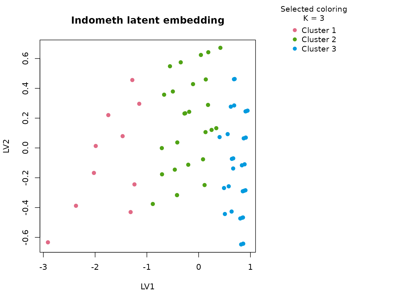

plot_consensus_heatmap(fit_ind, main = "Indometh consensus heatmap")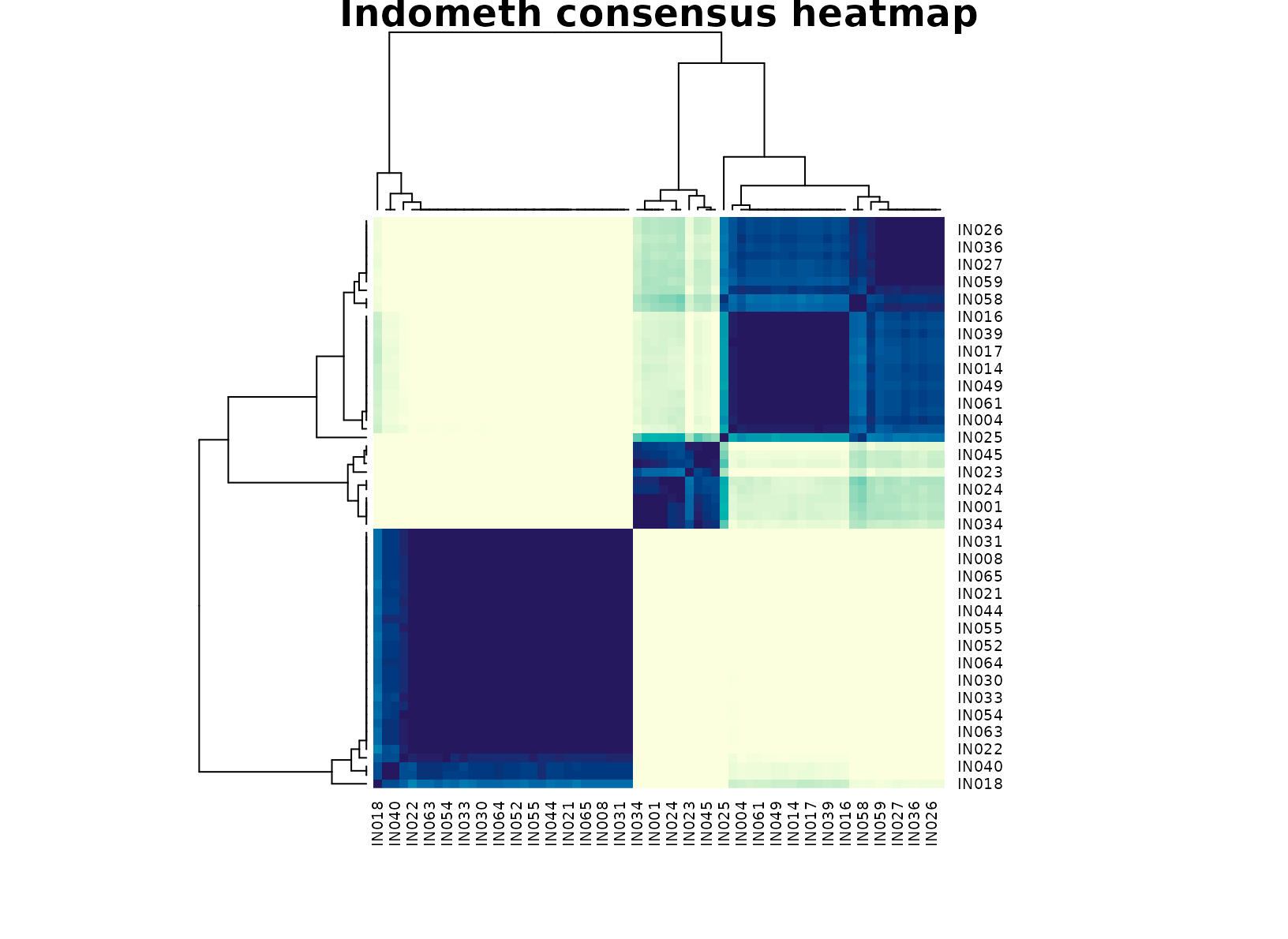

Discussion

The selected three-cluster solution is informative because the groups usually map onto different portions of the concentration trajectory. One cluster is typically enriched for early high-concentration points, one captures mid-curve measurements, and one collects lower concentrations later in the record. The time-band table makes that progression visible, but the subject table shows that no single subject owns a cluster outright. In other words, the partition is about recurring pharmacokinetic regimes rather than patient identity alone.

That matters in practice. A subject-only clustering would mostly summarize who was measured, while a pure time split would add little beyond the original study design. The consensus result is more useful because it compresses the table into interpretable concentration states that remain stable across resamples.

Interpretation

For Indometh, the clusters should be interpreted as descriptive concentration regimes spanning early absorption, transition, and later elimination-like behavior. The package is not fitting a compartment model, so the output should not be over-read as mechanistic PK inference. Its value is that it produces a stable exploratory stratification of the repeated-measures table that can be used for review, faceting, or downstream diagnostics.